programming · compilers · mlir
When a Loop Becomes an Integer Problem: Presburger Reasoning in MLIR Affine
How MLIR models affine loops with integer constraints to answer dependence, projection, and transformation-legality questions.
Suppose I want to parallelize this loop:
affine.for %i = 0 to %N {
  %x = affine.load %A[2 * %i] : memref<?xf32>
  affine.store %x, %A[2 * %i + 1] : memref<?xf32>
}
Assume %A has room for elements. Every iteration reads an even address
and writes the following odd address. Because both accesses use the same memref
and one of them writes, dependence analysis must ask whether two distinct,
ordered iterations can touch the same element.
To compare two executions of the loop, call the earlier iteration and the
later iteration . They are two possible values of the loop variable %i.
For any iteration , the read and write addresses are
A loop-carried flow dependence, also called a read-after-write dependence, would require the earlier write address to equal the later read address :
Over the rationals, satisfies the access equality. Over the integers, it is impossible: the left side is odd and the right side is even. The reverse load-to-later-store pair would require , which is impossible for the same reason. Two stores select the same address only when , contradicting . The flow, anti, and output dependence candidate sets are therefore empty, so these memory accesses do not block parallelization.
MLIR’s Affine dialect is useful because the compiler can recover this problem
from the program. Affine is not merely a nicer spelling of a for loop. Its
restrictions preserve enough mathematical structure for a question about
program order and memory indices to become a question about integer sets and
relations. The syntax is a contract; integer reasoning is what the compiler gets
in return.
We will follow that reasoning from Affine syntax to access relations, matrix constraints, and an emptiness result.
Two evidence sources are used below. Command transcripts were produced with the
Homebrew mlir-opt binary from LLVM 22.1.4. Implementation links and source
descriptions are pinned separately to LLVM revision
07aa3b7;
the local binary was not built from that revision.
What Affine promises
The Affine dialect documentation separates identifiers into dimensions and symbols. Dimensions are coordinates of the object being described: loop induction variables, tensor indices, or the input tuple of a map. Symbols are fixed but unknown parameters for the relevant affine scope.
#index = affine_map<(d0)[s0] -> (2 * d0 + s0)>

%address = affine.apply #index(%i)[%N]
In the application, %i supplies dimension d0 and %N supplies symbol s0,
so %address represents 2 * %i + %N. Calling %N a symbol does not mean its
value was known at compile time. It means the analysis may treat one
invocation’s %N as invariant while dimensions vary.
An affine map returns one or more affine expressions. An affine integer set is a conjunction of constraints:
#inside = affine_set<(d0)[s0] :
  (d0 >= 0, -d0 + s0 - 1 >= 0)>

affine.if #inside(%i)[%N] {
  // 0 <= i < N
}
Surface IntegerSet syntax is consequently smaller than the full language of
Presburger arithmetic. It has one conjunction, not arbitrary nested unions and
complements. MLIR also defines semi-affine expressions, which admit symbolic
multipliers and divisors, but that larger grammar does not guarantee that every
Affine operation or analysis can flatten every such expression. Syntax,
internal representation, and supported analysis are three different
boundaries.
The restrictions are enforced. With the Homebrew mlir-opt binary, version
22.1.4, this complete stdin input reproduces the verifier check:
mlir-opt - <<'MLIR'
#not_affine = affine_map<(d0, d1) -> (d0 * d1)>
module {}
MLIR
It reports:
<stdin>:1:42: error: non-affine expression: at least one of the multiply operands has to be either a constant or symbolic
#not_affine = affine_map<(d0, d1) -> (d0 * d1)>
                                         ^
Both operands vary as dimensions, so the product is outside the contract. There is no coefficient matrix for with constant coefficients.
Failure to satisfy a constraint is different from failure to satisfy the IR rules. The same tool accepts the contradictory set below. Canonicalization then proves the guarded branch unreachable:
mlir-opt --canonicalize - <<'MLIR'
#empty = affine_set<(d0) : (d0 >= 0, d0 <= -1)>

module {
  func.func @valid_but_empty(%i: index) {
    affine.if #empty(%i) {
      %unused = arith.constant 0 : i32
    }
    return
  }
}
MLIR
Its output contains no affine.if:
module {
  func.func @valid_but_empty(%arg0: index) {
    return
  }
}
The variable product is invalid IR. The contradictory set is valid IR describing no integer points. An emptiness result is often the successful answer to an analysis, not a verifier error.
Iterations become memory relations
Sets answer when a statement executes. Relations answer what an execution
touches. An access relation is a set of (iteration, address) pairs. Using
for a store execution and for a load execution, the opening loop
has
The arrow separates an iteration coordinate from a memory coordinate. For this store-to-load pair, a dependence candidate exists when the write and the later read map to the same address:
The term comes from the loop’s sequential schedule. For this loop the schedule function is simply
so “the write executes before the read” becomes . In a nested loop, a schedule such as uses lexicographic order instead, but it still contributes integer order constraints to the same relation.
Eliminating leaves , or . The equality’s
coefficients have greatest common divisor 2, which does not divide 1, so the
integer set is empty. For this access pair, that proves NoDependence.
Mathematically, a sample from a nonempty set would be a concrete conflicting
pair. The routine below does not request one; it asks whether emptiness can be
established.
In LLVM source at revision
07aa3b7,
Affine dependence analysis follows this structure in code. It builds an access
relation for each operation, composes one with the inverse of the other, adds
source-before-destination ordering constraints, and checks whether the result
is empty. The same-memref and common-scope checks, plus domain construction,
occur earlier in the function. Reduced to the essential relation operations,
checkMemrefAccessDependence
looks like this:
if (failed(srcAccess.getAccessRelation(srcRel)) ||
    failed(dstAccess.getAccessRelation(dstRel)))
  return DependenceResult::Failure;

dstRel.inverse();
dstRel.mergeAndCompose(srcRel);
dstRel.convertVarKind(VarKind::Domain, 0, dstRel.getNumDomainVars(),
                      VarKind::Range, 0);
IntegerPolyhedron dependenceDomain(dstRel);
addOrderingConstraints(srcDomain, dstDomain, loopDepth, &dependenceDomain);

if (dependenceDomain.isEmpty())
  return DependenceResult::NoDependence;
return DependenceResult::HasDependence;
The asymmetry matters. NoDependence is conclusive. HasDependence means the
constructed relation was not proven empty, so a legality decision must
conservatively respect it; it does not promise that this routine produced a
concrete sample. Failure means the routine could not construct a supported
query.
At that source revision, checkMemrefAccessDependence immediately returns
NoDependence when two accesses use different memref SSA values. That is an
identity check, not a general alias analysis: the routine does not establish
whether distinct memref values refer to overlapping storage, and it does not
summarize unknown side effects. A compiler pipeline that needs those answers
must obtain them separately. For supported same-memref accesses that reach
relation construction, Presburger constraints answer whether their indices
meet in the forbidden execution order.
The geometry is useful; the lattice is the program
The opening dependence equality has rational solutions but no integer ones. That distinction begins with the iteration domain. For one loop,
is its iteration domain. %N may be unknown while compiling, so this is a
family of domains parameterized by , not one fixed interval.
A nested loop gives a two-dimensional domain. The explicit map on the inner lower bound matters in Affine syntax because the outer induction variable is a dimension, not a symbol:
affine.for %i = 0 to %N {
  affine.for %j = affine_map<(d0) -> (d0)>(%i) to %M {
    // 0 <= i < N and i <= j < M
  }
}
For fixed and , its inequalities draw a polygon. The actual executions are only the integer points inside it.
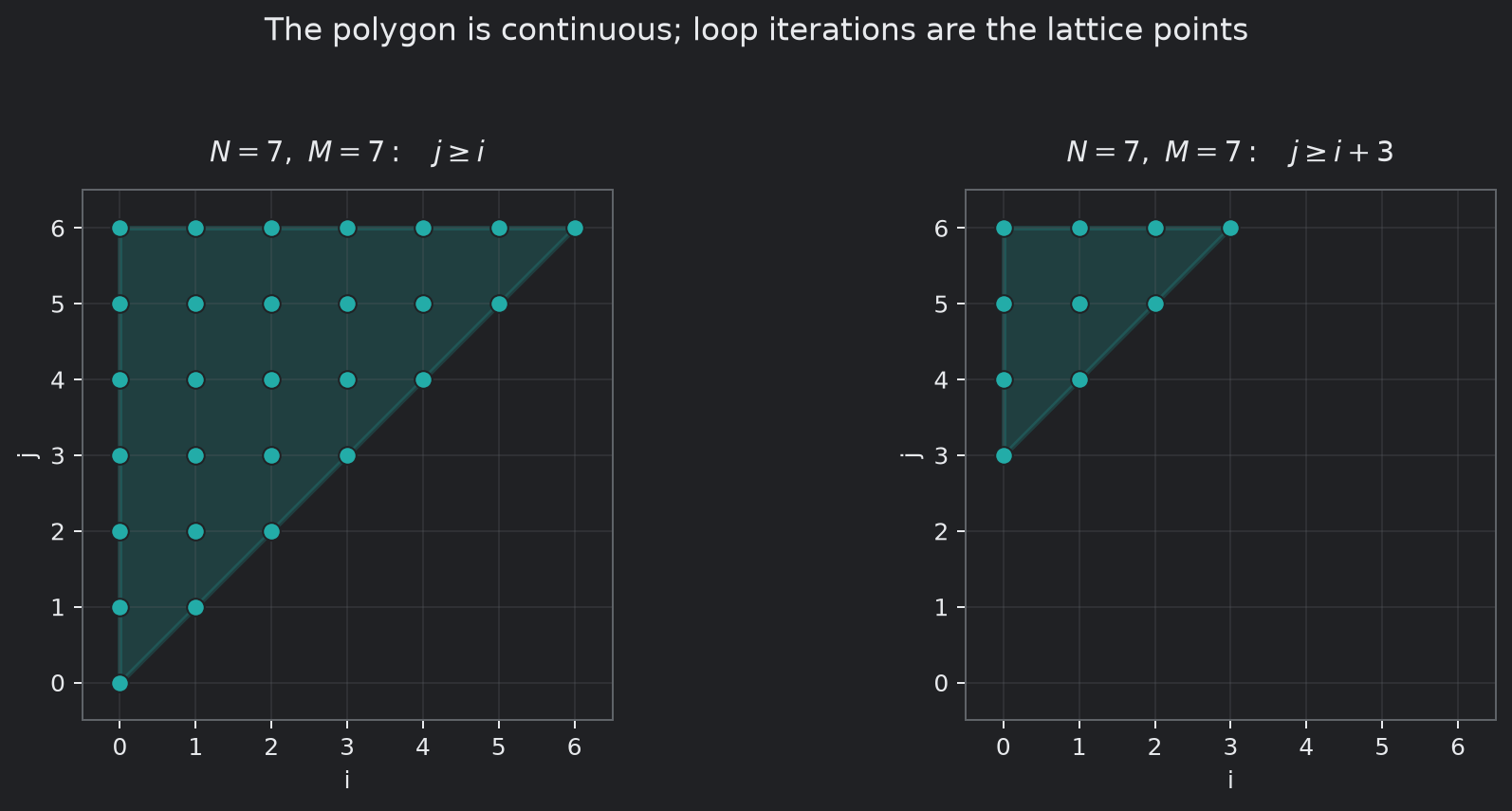
A continuous relaxation is useful geometry, but only the lattice points are loop iterations.
That distinction is not cosmetic. Set ; then the opening equality becomes
Over the rationals it has the solution . Over the integers it has none: the left side is always even.
A rational linear program can therefore say “feasible” when there is no program iteration at all. A convex polyhedron is a region in a real vector space, usually described here with integer or rational coefficients. Compiler iteration domains are the integer points in that region. “Polyhedral” and “Presburger” are related descriptions, not interchangeable words.
Presburger arithmetic is the first-order theory of integers with addition and order. It allows integer constants, Boolean connectives, and quantifiers. Multiplication by an integer constant is allowed: is repeated addition. Multiplication of two arbitrary variables, , is not.
Mojżesz Presburger proved the theory decidable in 1929. “Decidable” only says that an algorithm eventually answers every formula; it does not say the algorithm is cheap. Roughly, Cooper-style quantifier elimination removes one integer variable at a time by replacing its quantified constraints with a finite disjunction of boundary and residue cases. Repeating that process can make the formula grow rapidly, and the known lower bounds for unrestricted Presburger formulas are severe. Compiler analyses remain practical by exploiting program structure and asking narrower questions, rather than relying on decidability alone.
One conjunction of linear inequalities describes one convex region. Full Presburger formulas can also use disjunction, negation, quantification, and divisibility. Their solution sets are exactly the semilinear sets: finite unions of periodic linear pieces. This is why “a Presburger set is a polyhedron” is too strong. One polyhedron in the visible -space is an important case, but it cannot by itself describe, for example, every even integer. Add an existential witness , however, and describes exactly the evens: projection can leave a periodic integer set even when the higher-dimensional rational relaxation is one convex polyhedron.
Flattening syntax into rows
Return to the triangular loop domain:
Over integers, strict upper bounds become non-strict inequalities with a one-unit adjustment:
Put the variables in the order , append a constant column, and each inequality becomes one row:
Every row denotes its dot product with constrained to be
nonnegative. Equality rows use the same layout and are constrained to equal
zero. This is the convention used by
IntegerRelation.
The useful correspondence is the data model, not a reimplementation of MLIR in
another language. MLIR’s
SimpleAffineExprFlattener
also produces coefficient vectors ordered as dimensions, symbols, locals, then
the constant term.
FlatAffineValueConstraints
adds Affine-operation helpers and associations with SSA values on top of the
linear constraint structures. After flattening, adding constraints,
intersecting domains, or asking for a bound is matrix work rather than syntax
tree interpretation.
Addition and multiplication by constants flatten directly. Division is where the integer model has to retain information that a rational approximation would erase.
The constraint data model
There is no pass that lowers an affine.for into one of these types. They are
temporary analysis data structures, not stages in a lowering pipeline. Three
types are enough to follow the path used in this article:
| Type | Role |
|---|---|
IntegerRelation | Stores one conjunction of equality and inequality rows over domain dimensions, range dimensions, symbols, and existential locals. |
IntegerPolyhedron | Provides the set-shaped form, with set dimensions instead of separate input and output tuples. |
FlatAffineValueConstraints | Adds helpers that read Affine operations. Through its base class, it can associate an optional SSA value with each non-local variable. It inherits the set-shaped constraint storage rather than being converted into it. |
For the triangular loop, Affine helpers add the bounds to the set-shaped
constraint object. The result is the four-row matrix shown earlier, with %i
and %j attached to set-dimension columns and %N and %M attached to symbol
columns. For an access relation, the same library instead uses an input tuple
for the iteration and an output tuple for the accessed index. In both cases,
PresburgerSpace records the role of every variable column.
The client then asks its question. Dependence analysis adds execution-order
constraints and tests emptiness. A client that requests a sample receives a
concrete integer witness rather than just true. The Affine operations and
attributes remain in the IR while this temporary analysis state is created and
discarded.
Integer emptiness and sampling
Integer feasibility is not ordinary linear-program feasibility with a different
name. IntegerRelation::isEmpty
can prove emptiness using variable elimination and divisibility checks. For
, the equality’s coefficients have greatest common divisor 2, which
does not divide 1, so the integer set is empty even though its rational
relaxation contains .
Finding a witness is a separate operation. For bounded sets,
Simplex::findIntegerSample
searches for an actual integer point. A rational tableau point is not returned
as an integer sample.
Nothing in this path requires sending every Affine query to an external SMT solver. MLIR contains dedicated constraint representations, elimination routines, integer sampling, and set operations. That does not make the problems inexpensive; it makes the implementation and its supported fragments explicit.
Projection leaves a remainder
Take the integer relation
Projecting away asks which values have some integer witness :
Project the corresponding line over the rationals and every rational survives: choose . Integer projection leaves a congruence condition. This is the point usually lost when Presburger reasoning is summarized as “linear inequalities.”
MLIR can retain the witness as a local variable. For a positive constant , let
The quotient is characterized by
or, in MLIR’s nonnegative-row convention,
The remainder is then . At the pinned source revision, flattening does
exactly this for constant floordiv and mod: it introduces the quotient as a
local and adds the bounding inequalities. The surface program can remain
compact:
#floor = affine_map<(d0) -> (d0 floordiv 4)>
#remainder = affine_map<(d0) -> (d0 mod 4)>

%q = affine.apply #floor(%i)
%r = affine.apply #remainder(%i)
Internally, locals follow dimensions and symbols in the coefficient columns.
PresburgerSpace
defines them as existentially quantified variables. An assignment to the
visible dimensions and symbols belongs to the set if some assignment to the
locals satisfies the rows. The hidden quotient is therefore not temporary
compiler bookkeeping with no semantics; it is the witness that preserves
division and congruence over the integers.
Tiling as coverage and uniqueness
The same integer-set vocabulary can describe the domain obligation for a loop transformation.
For a one-dimensional loop tiled by a positive constant , introduce a tile coordinate :
Projecting away should recover precisely
Coverage is not enough by itself. We also want every to have one tile owner, not several. The witness is
This value is a multiple of , and the definition of floor gives , so every original iteration has a tile. If two multiples of both owned , their difference would be a multiple of with magnitude less than . The difference must therefore be zero, which proves that the owner is unique.
The transformation is reproducible from a complete empty loop nest, which isolates the domain change from the loop body:
mlir-opt --affine-loop-tile='tile-sizes=4,4' - <<'MLIR'
module {
  func.func @domain(%n: index, %m: index) {
    affine.for %i = 0 to %n {
      affine.for %j = 0 to %m {
      }
    }
    return
  }
}
MLIR
The documented
affine-loop-tile
pass in the Homebrew mlir-opt 22.1.4 binary produces the following loop-bound
excerpt:
#map = affine_map<(d0) -> (d0)>
#map1 = affine_map<(d0)[s0] -> (d0 + 4, s0)>

affine.for %arg2 = 0 to %arg0 step 4 {
  affine.for %arg3 = 0 to %arg1 step 4 {
    affine.for %arg4 = #map(%arg2) to min #map1(%arg2)[%arg0] {
      affine.for %arg5 = #map(%arg3) to min #map1(%arg3)[%arg1] {
      }
    }
  }
}
The outer loops move by four. The inner upper-bound map returns both
tile-start + 4 and the original extent; min selects the boundary for a
partial final tile. The pass implementation at the pinned source revision is in
LoopTiling.cpp.
Coverage and unique ownership prove that the tiled domain neither drops nor duplicates an iteration. They do not by themselves prove transformation legality. Tiling may change execution order, so dependences and side effects remain separate obligations. The actual pass looks for tileable loop bands; the standalone formula only explains the domain part of its job.
Where the Affine contract stops
It is easy to leave this topic with an overly broad mental model: Affine is where MLIR loops live, and Presburger analysis optimizes all of them. Neither part is true.
scf.for expresses structured
iteration, but its SSA bounds do not necessarily satisfy Affine’s dimension and
symbol rules. SCF can preserve a loop shape without promising that its bounds
and accesses flatten into the matrices used here. There is a best-effort
raise-scf-to-affine pass, and its documented preconditions are evidence of
the difference rather than a way to erase it.
Affine maps also appear outside affine.for, including as indexing maps on
linalg.generic. More broadly,
there is no canonical pipeline in which every program travels through Tensor,
Linalg, Affine, SCF, Vector, GPU, and LLVM in one fixed order. Different
compilers preserve, introduce, or discard these contracts at different points.
Even inside Affine, one analysis may support less than the dialect can express.
At the pinned source revision, the dependence routine returns Failure, for
example, when two accesses lie in different Affine scopes, have no common block
within an Affine scope, or cannot be converted into access relations. That is
why Failure remains distinct from either dependence result.
Return to the loop at the beginning. It first looked like control-flow syntax. After exposing the contract, it has an iteration domain, a write relation, a read relation, an execution-order constraint, and the impossible equality . The candidate dependence set is empty, so these memory accesses do not prevent parallelization.
That is the useful way to read the Affine dialect. Its restrictions do not make compiler reasoning automatic or universally cheap. They keep particular questions decidable and present in the IR long enough for the compiler to ask them. When a program leaves the contract, the correctness obligation does not disappear; this route to answering it does.
References
- MLIR Affine dialect and Affine pass documentation.
- LLVM implementation source pinned independently at
07aa3b7:PresburgerSpace,IntegerRelation,AffineStructures,AffineAnalysis, andLoopTiling. - Christoph Haase, “A Survival Guide to Presburger Arithmetic”, ACM SIGLOG News 5(3), 2018.
- David C. Cooper, “Theorem Proving in Arithmetic without Multiplication”, Machine Intelligence 7, 1972, pp. 91–99.
- Alex McKenna et al., “Bringing Presburger Arithmetic to MLIR with FPL”, IMPACT 2022.
- Sven Verdoolaege, “isl: An Integer Set Library for the Polyhedral Model”, ICMS 2010, pp. 299–302.